fahb - Optimising progression criteria in multi-site pilot trials assessing recruitment
Introduction
Recruiting participants into clinical trials is hard, and if we don’t manage to do it well then the whole trial is at risk. Without participants and the information they provide, treatment comparisons will be underpowered and we are unlikely to see a statistically significant result even if we are lucky enough to have found an intervention which really works. Trials which aren’t able to answer their primary research question represent a huge drain on valuable resources (money, time, and, crucially, participant engagement) which might be better deployed elsewhere, and can damage trust in the research process. We would like to identify these situations early on in the trials lifecycle and be able to shut down trials early if they are clearly not going to be able to recruit enough participants in a timely manner.
One common approach to this problem is to run a pilot trial and
examine recruitment there. An external pilot is a small study which
looks a lot like the main trial we hope to run, but in minature. An
internal pilot constitutes the first phase of the main trial. Either
way, the idea is that we can look at the pilot recruitment data and use
it to judge if the main trial should go ahead / continue running. We
have written an R package, fahb
(feasibiliy assessment using hierarchical Bayes), to
help trial teams do this well.
Making progress
By far the most common method to assessing feasibility with a pilot trial is to set up what we call progression criteria. These are a set of thresholds which all need to be met for us to be sufficiently sure that the main trial won’t fail to recruit. Different pilot trials will measure different things in the progression criteria, but there are some fairly common elements. When thinking about recruitment, the NIHR recommends we look at three things once the pilot has finished:
- the number of participants recruited;
- the number of sites opened to recruitment; and
- the rate of participant recruitment, per site-year.
The idea is that we calculate these three summaries and compare them against pre-specified thresholds, and move forward only if they all exceed these thresholds. This seems pretty sensible, but the difficulty comes when choosing these thresholds. We need to be careful, since if we make them too lenient then they will be surpassed too easily and we’ll see lots of infeasible studies progressing. But we also need to make sure they are not too harsh, in which case too many good trials would fail at the pilot stage even though they are actually perfectly feasible. We know from Mellor et al.’s work that researchers often don’t feel confident in choosing their thresholds, worrying that they are fairly arbitrary.
Quite apart from choosing good thresholds, we might well worry about the very form of this decision rule. Are these the right quantities to be measuring? Should they be combined by asking that all thresholds are met? What about a rule where we proceed in any of the thresholds have been met? We found in some previous work that some common progression criteria were so ill-suited to the job that you’d be better off making your decisions by tossing a coin, regardless of the specific thresholds used. Is that the case here, too?
Positives and negatives
What we really need is a way to take a suggested set of progression criteria thresholds and evaluate them. Then we can compare different suggestions and have a concrete way to choose the best one. One approach here is to think about the false positive and false negative rates which we obtain when applying a particular set of progression criteria thresholds. We call these the operating characteristics of the pilot trial.
By false positive rate, we mean the probability of getting a positive progression decision when in fact the trial is not going to recruit well. Conversely, the false negative rate is the probability of not getting a positive decision even though the trial is really feasible. But how do we calculate these measures?
One simple approach is to simulate some trials. Thinking about internal pilots for now, a trial simulation would generate a site opening and participant recruitment process according to an assumed statistical model. For that simulated trial we can make a note of how long it took until it hit its recruitment target, but also of the three pilot summary statistics described above. We can use the former to classify this trial as either feasible or infeasible by comparing the recruitment time to a threshold value which denotes the tipping point from feasible into infeasible. And we can compare the pilot summaries against our pre-specified thresholds to see if we would have progressed of stopped the trial early. This gives us two outcomes: the underlying feasibility of that simulated trial, and the progression decision made after the pilot phase.
We can repeat this many times and then use these simulated results to estimate our operating characteristics. We can get the false positive rate by looking at all the simulated trials which were really infeasible, and working out the proportion of these which decided to progress after the pilot. Similarly, the false negative rate is the proportion of all feasible simulations where we incorrectly decided to stop after the pilot. We can do this for different progression criteria thresholds, looking for some which give us a low false positive rate and a low false negative rate.
There’s something fishy about this model
We’ve proposed a particular model of site opening and participant
recruitment, to let us simulate all these hypothetical trials. For site
opening, we assume this proceeds randomly but with a consistent overall
rate - specifically, we model openings using a Poisson process. To
use fahb, the user needs to say something about what they expect the
opening rate of this process to be.
We assume a similar model for the recruitment of participants to sites -
that this will be random, but with a consistent rate. But we know that
the rate of recruitment can vary between different sites, with some
doing really well and others not so much. We capture this behaviour by
using a hierarchical model along the same lines as proposed by
Anisimov & Fedorov, who showed that these kinds of models fit well to
observed trial recruitment data. To use fahb the user needs to say
what they expect about the overall recruitment rate, and also how much
they expect the recruitment rates to vary between sites.
Deciding on decison rules
To use fahb we first set up a problem, then generate a set of
simulations, before finally looking for good progression criteria
thresholds. To generate the problem we need the model specification as
described above (we will use the package defaults here for illustration)
along with our recruitment target N, number of sites m, and time t
(in years) that we will analyse the internal pilot data at. For example:
library(fahb)

# Initialise the problem
problem <- fahb_problem(N= 320, m = 20, t = 0.5)

# Run n_sims simulations
problem <- forecast(problem, n_sims = 10^4)

# Look for good PC thresholds
design <- fahb_design(problem)
The results can be summarised by plotting the design:
plot(design)
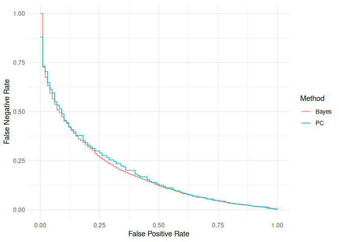
This graph shows us the operating characteristics (the false positive and false negative rates) of a range of different decision rules. Note that there are two methods here: “PC” are the standard progression criteria as described above, and “Bayes” are a different type of decision rule which involves a more complex analysis of the pilot data (for more information see the associated manuscript by Wilson et al.). We see that we need to trade off the false positive rate against the false negative rate, and how we do that will depend on our own individual priorities. We also see that the quality of decision rules using progression criteria is very close to the quality of those using the more involved Bayesian analysis - this gives us some confidence that the basic format of these rules is pretty well suited to the problem.
We can see the exact error rates and the corresponding progression criteria thresholds of all the decision rules illustrated here by printing the design:
design
## Standard progression criteria
##
##     FPR        FNR        n_p         m_p        r_p
## 1   0.0 0.88332170 15.9340644  5.99216607 10.4609405
## 11  0.1 0.47327285 10.1741878 -0.05009205  6.4552787
## 21  0.2 0.34919749  7.6107493  1.34276203  5.9792804
## 41  0.4 0.18325192  4.2499347 -0.53299157  5.1709904
## 51  0.5 0.12672715 -0.4801782 -0.67936391  4.9283610
## 71  0.7 0.05792045 -0.3246740 -0.97265220  3.6425854
## 81  0.8 0.03461270  0.7709202 -0.69947830  2.8415294
## 91  0.9 0.01926029 -0.8144763 -0.87928814  1.7437179
## 101 1.0 0.00000000 -0.4606959 -0.98219188 -0.3552817
##
## Bayesian approximation
##
##     FPR        FNR      T_p
## 1   0.0 1.00000000 1.088897
## 11  0.1 0.45429170 3.115605
## 21  0.2 0.34696441 3.268041
## 41  0.4 0.17739009 3.534804
## 51  0.5 0.12826239 3.649131
## 71  0.7 0.06043266 3.870856
## 81  0.8 0.03503140 3.992112
## 91  0.9 0.01158409 4.099511
## 101 1.0 0.00000000 4.546426
##
## FPR - False Positive Rate
## FNR - False Negative Rate
##
## n_p, m_p, r_p - Probabilistic thresholds for standard
##                 progression criteria on the number recruited,
##                 number of sites opened, and the recruitment rate
##                 (participants per site per year) respectively
##
## T_p - Bayesian decision rule threshold for the posterior predictive
##       expected time until full recruitment
By default this gives us the rules which give us FPRs of
$0, 0.1, \ldots , 0.9, 1$, but you can see a finer grained version by
using print.fahb_design(design, coarse = FALSE). Once we have decided
on what kind of balance between the OCs we are happy with, we can read
of the associated progression criteria thresholds and use them for our
pilot.
One thing that’s interesting here is that we often see good progression criteria which have one (or sometimes even two) negative thresholds. In practice this means the threshold will always be exceeded, so it ends up being a redundant part of the decision rules and we can just forget about it. This suggests that we might often miss out on the best progression criteria thresholds if we ask that all three components are specified, as the NIHR do.
Seeing the future
If we are using pre-specified progression criteria then analysis of the
pilot data is straightforward - we just calculate the three summary
measures and compare them against the thresholds we have chosen,
progressing if all of the thresholds are exceeded. We can also use
fahb to run a Bayesian analysis of the recruitment data and provide a
predictive distribution, conditional on what we have observed in the
pilot, of the time needed to hit our recruitment target. To do this we
need to provide the pilot recruitment data in for the form of a vector
n_pilot of recruitment numbers at each open site, and a corresponding
vector t_pilot of how long (in years) these sites have been open.
Because this function runs a Bayesian analysis using Stan, it needs to
first compile the associated Stan code and this can take a bit of time.
Once this has been done, if you want to run the analysis again you can
extract the compiled model and provide it to another call of
fahb_analysis so it can be re-used.
fahb_analysis(n_pilot = c(1,4,3),
              t_pilot = c(0.43, 0.2, 0.07),
              problem)
## Compiling the model...

## the number of chains is less than 1; sampling not done

## Standard progression criteria statistics:
##      n_p      m_p      r_p
##  8.00000  3.00000 11.42857
##
## Expected posterior predictive time to recruit:
## exp_pp_T
## 3.011657
##
## Posterior predictive distribution quantiles:
##     0.5%     2.5%      20%      50%      80%    97.5%    99.5%
## 1.928465 2.120365 2.546714 2.951318 3.438331 4.231460 4.786017
##
## Posterior site opening rate hyperparamaters (Gamma):
## shape  rate
## 33.00  3.35
We can then use this predictive distribution to decide if the trial
should continue or not, either by making a judgement directly or by
applying a pre-specified threshold for the expectation of this predicted
time as suggested by the fahb_design object.
Size matters
We can use fahb to design and analyse external pilots, too. The main
difference at the design stage is that we need to specify how many sites
to have in the pilot (m_ext), and the target recruitment (n_ext). We
still set a time t for the pilot analysis, which now acts as a
maximum: we will stop the external pilot when we hit the target pilot
recruitment or at time t, whichever comes first.
The operating characteristics of an external pilot are going to be
impacted by its sample size, so we can use fahb to explore this and
help us choose how many sites and participants to recruit. For example,
let’s compare two pilots recruiting 60 participants over 1 year, but
with one using 3 sites and the other using 10. We will focus on decision
rules of the standard progression criteria form.
library(ggplot2)

problem <- fahb_problem(N = 320, m = 20,
                        t = 1, n_ext = 60, m_ext = 3)
problem <- forecast(problem)
design_m3 <- fahb_design(problem)

problem <- fahb_problem(N = 320, m = 20,
                        t = 1, n_ext = 60, m_ext = 10)
problem <- forecast(problem)
design_m10 <- fahb_design(problem)

# Put the OCs of the two designs into a data frame for plotting together
df <- rbind(design_m3$Prog_Crit_OCs, design_m10$Prog_Crit_OCs)
df$m <- factor(rep(c(3, 10), each = nrow(design_m3$Prog_Crit_OCs)))

ggplot(df, aes(x = FPR, y = FNR, colour = m)) + geom_step() +
  theme_minimal()
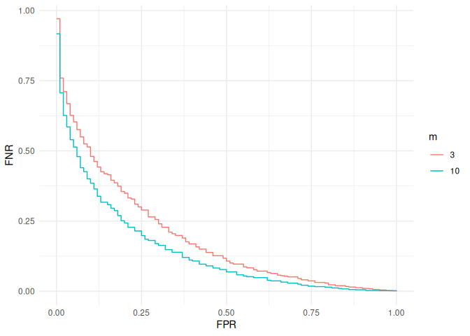
This shows what kind of benefit we could expect from increasing the
number of sites in the pilot. For example, if we wanted a false positive
rate of 0.2, increasing from 3 to 10 sites would bring the false
negative rate down by around 0.1. We could continue in this manner to
look at other choices for n_ext, m_ext and t until we find the right
balance.
Green-lighting progression criteria
In fahb we have provided one potential solution to the problem of
choosing good progression criteria thresholds, and of choosing other
aspects of pilot trial design such as the timing of an internal pilot or
the sample size of an external one. We have also shown that progression
criteria based on the three summary measures suggested by NIHR can be of
high quality, in the sense that they lead to operating characteristics
almost as good as decision rules based on a full Bayesian analysis of
the pilot data. This all means that if we are happy with the modelling
assumptions encoded in fahb, we can safely use it to determine good
progression criteria which give the desired balance between the risks of
false positives and false negatives, making them less arbitrary and more
defensible.
Further work
To extend this work further, it would be nice to consider other models of the recruitment process. For example, we may anticipate a less variable pattern of site opening than the Poisson process we have assumed would give; or we may even want to model a fully deterministic process where we set up a plan for site opening and assume it will be adhered to exactly. Other approaches to modelling like those surveyed by Gkioni et al. could also be considered. A modular approach could be explored to allow for different models for site opening and for participant recruitment to be mixed and matched. If we were to use different models, we would need to check if the same qualitative results hold - i.e. if standard progression criteria are still able to provide good decision rules when compared to Bayesian alternatives.
Before any of that, the priority should probably be helping people
determine the model inputs required to use fahb - something we have
glossed over a little here by just using the function defaults. These
inputs define the prior distributions of the three model parameters,
and they could be determined by using historic data, through expert
elicitation, or some mixture of both. This will likely need some more
methodological research; for example, working out the best way to elicit
expert beliefs around likely site recruitment rates and the variability
between them.
References
- Anisimov, V.V. & Fedorov, V.V. (2007). Modelling, prediction and adaptive adjustment of recruitment in multicentre trials. Statistics in Medicine 26(27), 4958–497.
- Gkioni, E., Ruis, R., Dodd, S. & Gamble, C. (2019). A systematic review describes models for recruitment prediction at the design stage of a clinical trial. Journal of Clinical Epidemiology 115, 141-149.
- Mellor, K., Dutton, S. J., Hopewell, S. & Albury, C. (2022). How are progression decisions made following external randomised pilot trials? A qualitative interview study and framework analysis. Trials 23(123).
- Wilson, D.T., Cowtan, S., Vyner, C. (2026). Optimising progression criteria in multi-site pilot trials assessing recruitment.