tout - Optimal design for trials with three outcomes
Introduction
Clinical trials aim to inform decisions. One of the clearest ways that can happen is through a hypothesis test, where we calculate a statistic summarising the trial data and compare it to a threshold value. If the statistic is greater than the threshold we reject our null hypothesis and make a positive decision (like proceeding to the next phase of evaluation); if it’s lower, we don’t reject the null and we make a negative decision (like stopping any further evaluation of the treatment).
There’s a clear tension between the simplicity and rigidity of this kind of procedure and the nuances of real-life decision-making. For that reason, some people have suggested we build some flexibility into our hypothesis test by using two thresholds. We make positive and negative decisions when the statistic lands above (below) the largest (smallest) of these, but if the statistic lands in between them we do something else: we allow ourselves the freedom to make our decision ourselves, and not have it dictated by the result of the test.
This has some intuitive appeal: it means that if we get a really clear result in either direction we will follow the result of the test, but if we get something less conclusive we can think about things carefully and try to work out what to do. We do this a lot in pilot trials, which commonly specify a “traffic light” system for assessing a given quantity - we then take our estimate from the pilot and see if it falls in the “red”, “amber”, or “green” region and act accordingly. But how do we choose these regions / thresholds? Although this is very much a statistical problem, there has been remarkably little analysis of this problem from a statistic perspective. Having recently examined other aspects of pilot trial decision rules (Wilson et al. 2021), we were interested to see if we could use a formal framework to help us decide what thresholds are optimal when using these kinds of traffic light decision rules.
Three-outcome designs
Fortunately, there were already some formal frameworks we could look at. These were proposed in the context of early phase drug trials, rather than pilot trials, but should be easy enough to translate across. One framework was proposed back in 2001 by Sargent et al.. They approached the problem by thinking about the operating characteristics of the trial. They defined four of these - the probabilities of:
- a “go” outcome under the null hypothesis;
- a “pause” outcome under the null hypothesis;
- a “stop” outcome under the alternative hypothesis; and
- an “pause” outcome under the alternative hypothesis.
Denoting these probabilities by $\alpha, \lambda, \beta$ and $\delta$ respectively, we can visualise them as areas under the sampling distribution densities when the null and alternative hypotheses hold:
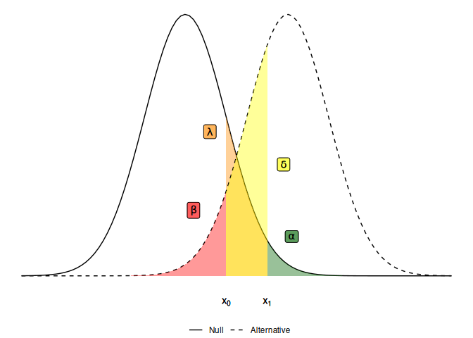
The idea is that we want these probabilities to be small, because ideally we want a “stop” outcome (where our statistic is less than the lower threshold $x_0$) under the null and a “go” outcome (where our statistic is greater than the upper threshold $x_1$) under the alternative. To find optimal thresholds $x_0$ and $x_1$, and an optimal sample size for the trial, we can set some constraints on each of these operating characteristics and find the smallest trial design which satisfies those constraints.
So far, so good - it looks like we can use this established method for phase II trial design to help us optimise pilot trials. Moreover, the 2001 paper suggests that adding this intermediate outcome will reduce the sample size needed, when compared against a typical two-outcome alternative. And this feels intuitive: by introducing this intermediate outcome we have a trial that is less decisive, so it seems natural that it will need less information. But a closer inspection reveals that this is not the case and in fact, the opposite is true - if we want to include an intermediate outcome in a trial, we will need to pay for that by increasing the sample size.
Making mistakes
To see why this is the case, we need to think about what these operating charactersics represent. The quantity $\alpha$ should be analogous to the type I error rate - the probability of making a positive conclusion under the null. In our pilot trial context, a positive conclusion means deciding to go ahead and run a large, definitive trial. Similarly, $\beta$ should be akin to the type II error rate - the probability of a negative conclusion (for us, deciding against a large definitive trial) when the alternative hypothesis actually holds. But these interpretations are not quite right.
Really, $\alpha$ only tells us the probability of making an immediate mistake under the null hypothesis. But there is another way to make that same mistake - we could land in the intermediate zone and then, free to make the decision ourselves, incorrectly decide we should progress to the next trial. This will still be a type I error because we are still under the null hypothesis - the true parameter value is still so poor that we don’t want to proceed, immediately or otherwise. Likewise, $\beta$ gives us the probability of an immediate false-negative, but does not account for the false-negatives we can arrive at via an intermediate outcome.
A new framework
We wanted to re-define the operating characteristics for a three-outcome design to recognise that false-positive and false-negative decisions can be arrived at in two ways: immediately, and following an intermediate outcome. This then let’s us make a fair comparison between two-outcome and three-outcome designs, because their operating characteristics now mean the same thing.
We introduced a simple model to describe decision-making after an intermediate outcome, supposing that the decision-maker will have a certain probability of making a mistake. In simple scenarios where the data tell us everything there is to know about the quantiy we’re trying to measure, we will only be able to take a random guess at what we should do - so the probability of making a mistake will be 0.5. We also needed to introduce another operating characteristic to let us control how likely we are to land in the intermediate region. We take the same approach as Storer did back in 1992 and introduce $\gamma$ - the probability that we land outwith the intermediate outcome zone (and thus make an immediate decision) when the true parameter value is halfway between the null and the alternative hypothesis. This new framework then sits as a reformulation of Storer’s approach, with Sargent et al.’s method being a special case.
Implications for sample size
Having worked out how to calculate these operating characteristics (see
our 2024 paper for details on these), we wrote the package tout to
find optimal (i.e. smallest) trial designs subject to constraints. For
example, suppose we are looking at a binary endpoint with a probability
$p$. If our null hypothesis is $p = 0.2$ and our alternative is
$p = 0.4$, constraining $\alpha \leq 0.1$ and $\beta \leq 0.2$ gives:
library(tout)

tout_design(rho_0 = 0.2, rho_1 = 0.4, alpha_nom = 0.1, beta_nom = 0.2)
## Three-outcome design
##
## Sample size: 24
## Decision thresholds: 7 7
##
## alpha = 0.08917126
## beta = 0.1919452
## gamma = 1
##
## Hypotheses: 0.2 (null), 0.4 (alternative)
## Modification effect range: 0 0
## Error probability following an intermediate result: 0.5 0.5
This tells us we need a sample size of 24, and that the two decision thresholds coincide at 7 - that is, the optimal three-outcome design is actually a two-outcome design. If we want a third outcome, we need to force it by constraining our third operating characteristic $\gamma$ to a level lower than the default of 1:
d <- tout_design(rho_0 = 0.2, rho_1 = 0.4, alpha_nom = 0.1, beta_nom = 0.2, gamma_nom = 0.5)
d
## Three-outcome design
##
## Sample size: 41
## Decision thresholds: 10 14
##
## alpha = 0.09623703
## beta = 0.1511409
## gamma = 0.498709
##
## Hypotheses: 0.2 (null), 0.4 (alternative)
## Modification effect range: 0 0
## Error probability following an intermediate result: 0.5 0.5
And we can visualise things by printing the tout object, which will
plot the sampling distributions under the null and alternative
hypotheses and shade them in according to the decisions made.
plot(d)
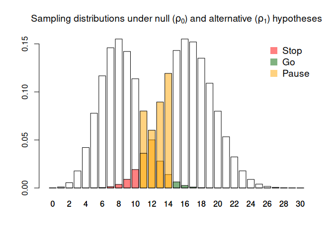
We see that in order to get this intermediate zone (here defined by a lower threshold of 10 and an upper threshold of 14), we need to pay for it through a larger sample size. This is because an intermediate outcome introduces volatility into the decision-making process, so we need more information to counteract that volatility and maintain our operating characteristics.
Post-pilot modifications
One of the main reasons we like to specify traffic-light decision rules in pilot trials is to give us a chance to improve things before the main trial. This might means making changes to the trial design, or the intervention, or both. But when we extend out formal framework to this kind of context we find that it becomes really difficult to find designs which still control our operating characteristics.
In tout we can signal that we plan to make post-pilot modifications by
specifying a range of modification effects; that is, we need to say a
priori what kind of shift in the parameter of interest we think we’ll
be able to achieve. For example, suppose we think our modification will
lead to an improvement of $\tau \in [0.05, 0.1]$:
tout_design(rho_0 = 0.2, rho_1 = 0.4, alpha_nom = 0.1, beta_nom = 0.2, gamma_nom = 0.5, tau = c(0.051, 0.1))
## Three-outcome design
##
## Sample size: 60
## Decision thresholds: 11 16
##
## alpha = 0.09009013
## beta = 0.185854
## gamma = 0.4505197
##
## Hypotheses: 0.2 (null), 0.4 (alternative)
## Modification effect range: 0.051 0.1
## Error probability following an intermediate result: 0.5 0.5
This increases our sample size by a factor of almost 50%. If we are less confident about how successful the modification will be, and reduce the lower limit to $0$, things get even worse:
tout_design(rho_0 = 0.2, rho_1 = 0.4, alpha_nom = 0.1, beta_nom = 0.2, gamma_nom = 0.5, tau = c(0, 0.1))
## Three-outcome design
##
## Sample size: 132
## Decision thresholds: 30 37
##
## alpha = 0.09740442
## beta = 0.194207
## gamma = 0.4942016
##
## Hypotheses: 0.2 (null), 0.4 (alternative)
## Modification effect range: 0 0.1
## Error probability following an intermediate result: 0.5 0.5
This behaviour reflects a pretty fundamental mis-match between the pre-specified nature of our three-outcome hypothesis test and the dynamic nature of post-trial modifications. In reality, after the pilot has concluded we may well be able to say what effect a modification will have with some confidence; but before the pilot, that will generally be very difficult. After all, one of the reasons we run a pilot trial in the first place is because we don’t know what kind of problems we are likely to see, let alone know what the best solutions to those problems will be. In that context, being able to predict the range of modification effects in advance with any degree of precision seems unrealistic.
Three-outcome designs - red, amber, or green?
Overall, our work paints a fairly dispiriting picture of three-outcome designs. We have shown that when we define our operating characteristics in a way that allows a fair comparison with two-outcome designs, we always need a larger sample size if we want to have that intermediate outcome. And we’ve found that one of the main motivations for that in the pilot trial context - to give us a chance at improving the trial based on what we saw in the pilot, rather than abandoning the intervention altogether - is not actually well-served by this framework of pre-specified decision rules.
So, are there any situations where we would want to use a three-outcome design?
For me, the most compelling argument is one given as motivation in
Sargent et al.’s paper - the fact that decisions about progressing
treatments on to the next stage of evaluation should not be completely
dictated by one outcome, but rather be based on a more complex analysis
which looks at the effect of treatment in several dimensions. Whenever
we find a treatment that isn’t terrible with respect to the primary
outcome, but equally isn’t amazing, being able to open up the
decision-making process to look at other outcomes seems really sensible.
And, as Sargent et al. argued, this is undoubtedly what happens in
practice when we end up with a borderline result. Acknowledging that
reality, we can use tout to find designs which still control the
operating characteristics we are interested in; but we need to prepare
for paying for the flexibility of a third outcome in the form of a
larger sample size.
Further work
The tout package was chiefly motivated by pilot trials, and as a
result is limited to single-arm hypothesis tests (common in pilots
looking at parameters like overall recruitment rates, retention rates,
or adherence rates in the intervention arm only). It would be useful to
extend the software to to the two-sample setting. This is currently
posted as an issue on the tout
repository. Any contributions to this issue, or to any other
improvements to tout, are very much welcome. If you would like to help
but aren’t yet familiar with using Git and GitHub to collaborate, get in
touch.
A major limitation of the frequentist three-outcome (and indeed two-outcome) framework in the pilot setting is it’s inability to deal with post-pilot modifications. One avenue of methodological research I’m exploring is how to model modification effects in a Bayesian framework; this let’s us avoid having to pre-specify decision rules, whilst accounting for uncertainty in the effect of modifications in a natural way. Please do get in touch if you’re interested in exploring these ideas.
References
- Sargent, D.J., Chan, V. & Goldberg, R.M. (2001). A Three-Outcome Design for Phase II Clinical Trials. Controlled Clinical Trials, 22(2), 117-125, https://doi.org/10.1016/S0197-2456(00)00115-X
- Storer, B. E. (1992). A Class of Phase II Designs with Three Possible Outcomes. Biometrics, 48(1), 55–60. https://doi.org/10.2307/2532738
- Wilson, D.T., Hudson, E. & Brown, S. (2024). Three-outcome designs for external pilot trials with progression criteria. BMC Med Res Methodol 24, 226. https://doi.org/10.1186/s12874-024-02351-x
- Wilson. D.T.,, Brown. J., Farrin, A.J., Walwyn, R.E.A. (2021). A hypothesis test of feasibility for external pilot trials assessing recruitment, follow-up, and adherence rates. Statistics in Medicine, 40, 4714-4731. https://doi.org/10.1002/sim.9091
- Wilson, D.T., Wason, J.M.S., Brown, J., Farrin, A.J., Walwyn, R.E.A. (2021). Bayesian design and analysis of external pilot trials for complex interventions. Statistics in Medicine, 40, 2877–2892. https://doi.org/10.1002/sim.8941